Overview of RStudio

Once installed, open up RStudio. You will see the console on your left, this is where you can type code and run R commands. There are two windows on your right, the top one shows you what is in the global R environment, and the bottom one is where you can view files, plots, packages and help pages.

There are two ways we can run R code in RStudio, directly from the console, or from an R script. We will start by looking at the console where we can write basic code to be run line by line.

Project management with Rstudio

In RStudio you can use “projects” to manage your files and code. These help by organising everything into a working directory and allowing you to easily keep your files, scripts and outputs for a single project in one place.

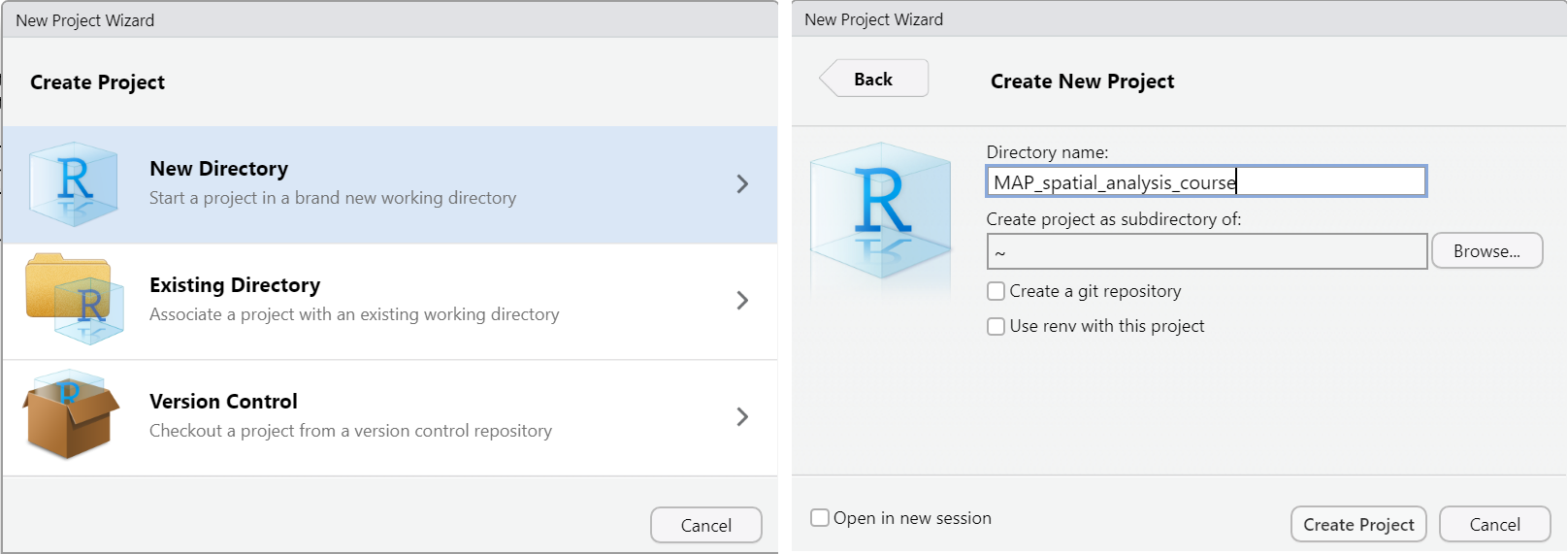
You can either create a new project from scratch in RStudio, create a project from an existing folder containing R code or by cloning a version controlled (e.g. Git) repository.

We will look at how to start a new project in RStudio. To do this we go to File > New Project. Select the option to create the project in a new directory and give the directory a name and create the project.

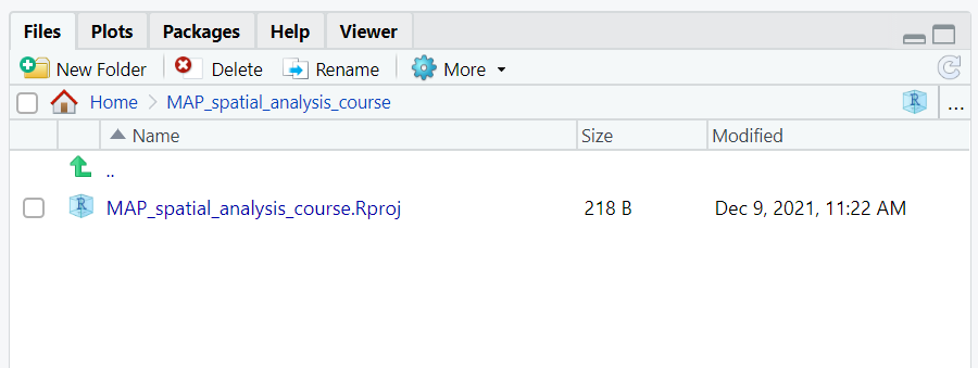
You will then see the project appear in the bottom right window. You can now navigate your project from this window. You can see the files you have saved as part of the project, create new folders, delete, move or rename files.

In this tutorial we will be working with the R project “NAME OF PROJECT” which can be downloaded from “WEBLINK TO DATA”.

Data types and structures

We will now introduce you to some of the basic data types in R. There are five main types of data in R, these are:

• Characters : “a”, “bananas”
• Numeric: 1 , 2.2321 , 1999
• Integer: 2L, 5L (L tells R to store as integer)
• Logical: True, False
• Complex: 1+4i (I is the imaginary part)
• Factors (categorical data with labels)

The major data structures in R are:

• Vectors
• Matrices
• Arrays
• Data frames
• Lists

Vectors are series of values, either numbers, characters or logical values (TRUE or FALSE).

Matrices are 2-dimensional array which can hold numeric, character or logical data types. All of the data in a matrix has to be of the same type and there is a fixed number of rows and columns.

A array is of 2 or more dimensions and as with a matrix can hold numeric, character or logical data types, with all data being of the same type

Data frames are a selection of equal length vectors grouped together, where the vectors can be of different data types. These are the most common format used to analyse datasets in and what we will primarily be working with in this session.

Lists are essentially a list of other items, these can be a mixture of different data types, for example you can create a list of data frames, matrices and vectors. It is useful way of organising and storing data.

Basic expressions

In the console we can write expressions and execute them by pressing enter. The most basic code we can write is simple calculations; when we press enter the calculation will be processed and a value returned.

5 + 5

## [1] 10

You can create variables and assign values to them, for example, we want to create a variable for the number of people tested for malaria. We want the variable to be called “tested” and for it to have the value of 120. We assign this using the <- sign. This will now appear in your global environment window on the top right. We can use the shortcut “alt and -” to input the<- sign.

tested <- 120

You can then refer to the variable in the code you write and it will work as the value assigned to it. It is then possible to do calculations based on this variable.

tested * 2

## [1] 240

tested / 10

## [1] 12

Creating another variable will allow us to perform calculations between those variables. These variables can then be updated and the same code rerun to produce updated results. For example, we received information telling us that of the 120 people tested for malaria, 80 were confirmed positive. We can assign this value to the variable “positive” and calculate the proportion of those tested who were confirmed positive.

positive <- 80
positive / tested  ## Proportion of people tested confirmed positive

## [1] 0.6666667

If we then received updated information that 160 people were tested, not 120, we can update the value for tested and recalculate the proportion of positive cases.

tested <- 160    
positive / tested 

## [1] 0.5

We can store the output value as a new variable and give it a name. This can then be called on from the environment.

proportion_positive <- positive / tested 
proportion_positive

## [1] 0.5

R isn’t restricted to numeric variables, we can also create variables of character strings in the same way.

country <- "Burkina Faso"
country

## [1] "Burkina Faso"

Vectors

In R we commonly work with vectors, these are sequences of values. Vectors can be numeric or character strings and are created using thec(), concatenate, function. Once we have created the vector we can access different values of the vector by using square brackets.[2] will return the second value in the vector.

tested <- c(56, 102, 65, 43, 243) 
tested[2]

## [1] 102

countries <- c("Burkina Faso", "Nigeria", "Tanzania", "Uganda")
countries[2]

## [1] "Nigeria"

Basic functions

Next we can run some functions in R. There are a range of base functions in R, and additional ones made available by installing “packages” (more details on this later). Functions often take arguments in brackets (). Some of the base functions in R allow us to easily compute common summary statistics on vectors. Here are some examples.

sum(tested)

## [1] 509

mean(tested)

## [1] 101.8

max(tested)

## [1] 243

Some functions will take additional arguments. Take theround() function. This takes two arguments, the first is the number you wish to round, the second is the number of digits to round to.

round(3.14159, 2)

## [1] 3.14

Scripts

In most situations you will be wanting to write multiple lines of reproducible code. To do this you can open an R script by going to File > New File > R Script (or the shortcut Ctrl+Shift+N). This opens a text editor in the top left window where we can write our code. You can then run the whole script by clicking the “Run” button. Alternatively, you can run sections by highlighting the lines to execute and either clicking “Run” or Ctrl+Enter. You can also run the script line by line, by typing Ctr+Enter to run the line your cursor is currently on. Scripts can be saved, shared with others, and built on or rerun at later dates. From this point on we will work in R scripts.

Installing packages

R has a range of base functions available to be used, these include things such as mean(), sqrt() andround(). For more advanced data management, analysis and visualisations there are additional packages you can download which contain a wide range of functions.

Many packages are available on CRAN. CRAN is “The Comprehensive R Archive Network” and it stores up-to-date versions of code and documentation for R. Packages from CRAN can be installed directly from RStudio. For this module we will primarily be using thetidyverse group of packages. First we need to install the packages, then we need to load it into R to be able to use the functions. At the top of most R scripts you will find code for the packages being used in that script.

install.packages("tidyverse")
library(tidyverse)

You will only need to install the package onto your machine once, from then on for each new session of R you will need to load the packages required, but not to install them again.

Help available in R studio

There is a range of help available in RStudio. The most basic and informative of these is the help() function or? operator. These provide access to the R help pages and documentation for the packages and functions. For example, if we look at the help page for the round(), which is a base R function, we can see a description of the function and the format the code needs to take.

?round

We can also access help pages for packages. This will show all of the help pages available for that package

help(package = tidyverse)

Alternatively many packages have vignettes. These are documents detailing the facilities in a package. They can be accessed from the help page of the project, as above, or called on directly.

vignette("pivot")

Finally, the internet provides a huge amount of help for coding in R. Search engines such as Google will provide multiple results for the problems you face (if you are struggling someone will have had the same problem before and asked for help!). Sites such as stackoverflow contain large numbers of questions and answers from the R users community.

Importing data

R has the functionality to import various types of data. One of the most common file types we work with are .csv files, but we can also import .dta files and .xlsx files among others.

We can import .csv files into RStudio using the base functionread.csv(). In this function we insert the file path to the data we wish to import. Note that as we have set up a project, this is our base directory so file paths stem from where the project is saved. We can assign the imported dataset to an object, here called “routine_data”, using the <- operator to store it in our environment.

For this module we are using a dataset called “routine_data”. This is an fake dataset of malaria routine case reporting and contains variables for the numbers of malaria tests performed and the numbers of confirmed cases. Data are reported by health facility for children under and over the age of 5 seperately.

routine_data <- read.csv("data/routine_data.csv") 

Other data types can easily be read into R using different packages available. Stata files (.dta) can be read in using theread_dta() function from the Haven package, and excel files (.xls or .xlsx) using the read_excel() function from the readxl package. Both of these packages are part of the tidyverse we installed earlier so they do not need to be installed, just loaded.

## Examples, not run
library(haven)
dta_file <- read_dta("filename.dta")

library(readxl)
excel_file <- read_excel("filename.xlsx")

Whilst read.csv() is the most common way to read data into R, there is the alternative read_csv() function (note the underscore). This is part of the tidyverse group of packages and is often a better option for reading in CSV files. This function is quicker, it reads the data in as a tibble instead of a data frame and allows for non standard variable namesm amongst other benefits.

routine_data <- read_csv("data/routine_data.csv") 

## Rows: 1200 Columns: 17
## ── Column specification ────────────────────────────────────────────────────────
## Delimiter: ","
## chr  (3): adm1, adm2, month
## dbl (14): hf, year, test_u5, test_rdt_u5, test_mic_u5, conf_u5, conf_rdt_u5,...
## 
## ℹ Use `spec()` to retrieve the full column specification for this data.
## ℹ Specify the column types or set `show_col_types = FALSE` to quiet this message.

There are various options we can use when importing data, such as whether to include headers, what character to use for decimal points, what to import as missing values. To explore these options you can look at the help pages e.g. ?read_csv.

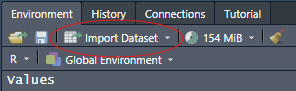
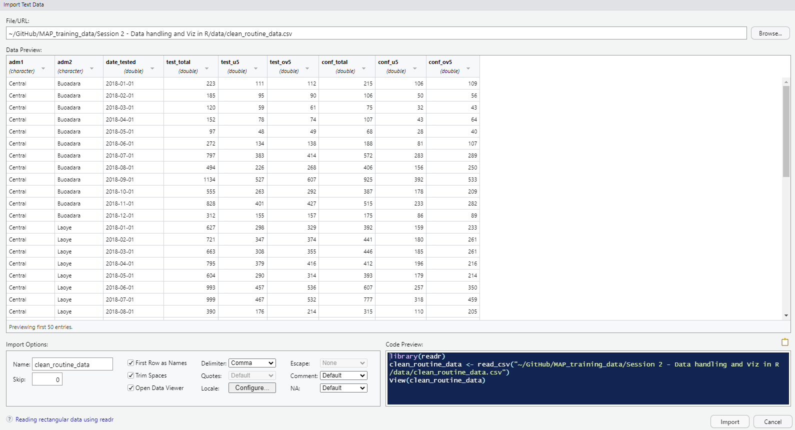
You can also use the interactive "Import dataset..." option above your Environment:  

Where with the "readr" package you can review your dataframe and specify which column contains which data type:

Data frames

We will now look at the csv we just imported. You will now see the “routine_data” object in your environment that we created and assigned this dataset too. You can see what the data looks like either by clicking on it in the global environment window or by typing the commandView(routine_data) which opens up a window displaying the data. Alternatively, we may just want to look at a few rows. We can do this by using the head() function, which shows us the first n rows of data

head(routine_data, 5)

## # A tibble: 5 × 17
##   adm1  adm2      hf month  year test_u5 test_…¹ test_…² conf_u5 conf_…³ conf_…⁴
##   <chr> <chr>  <dbl> <chr> <dbl>   <dbl>   <dbl>   <dbl>   <dbl>   <dbl>   <dbl>
## 1 West  Bamak…     6 Jan    2018     289     279     127     204     201       9
## 2 West  Bamak…     6 Feb    2018     178     175      87      92      90       4
## 3 West  Bamak…     6 Mar    2018      41      40      13      36      35       2
## 4 West  Bamak…     6 Apr    2018      NA     129      49      69      68       3
## 5 West  Bamak…     6 May    2018      95      93      28      64      62       4
## # … with 6 more variables: test_ov5 <dbl>, test_rdt_ov5 <dbl>,
## #   test_mic_ov5 <dbl>, conf_ov5 <dbl>, conf_rdt_ov5 <dbl>, conf_mic_ov5 <dbl>,
## #   and abbreviated variable names ¹​test_rdt_u5, ²​test_mic_u5, ³​conf_rdt_u5,
## #   ⁴​conf_mic_u5

To understand the structure of the data we can use thestr() command. This shows us that “routine_data” is a data.frame with 15 observations of 6 variables. The variables “country” and “method” are character strings, whilst “year”, “tested” and “confirmed” are integers and “mean_age” is numeric.

str(routine_data)

## spec_tbl_df [1,200 × 17] (S3: spec_tbl_df/tbl_df/tbl/data.frame)
##  $ adm1        : chr [1:1200] "West" "West" "West" "West" ...
##  $ adm2        : chr [1:1200] "Bamakiary" "Bamakiary" "Bamakiary" "Bamakiary" ...
##  $ hf          : num [1:1200] 6 6 6 6 6 6 6 6 6 6 ...
##  $ month       : chr [1:1200] "Jan" "Feb" "Mar" "Apr" ...
##  $ year        : num [1:1200] 2018 2018 2018 2018 2018 ...
##  $ test_u5     : num [1:1200] 289 178 41 NA 95 108 121 299 323 526 ...
##  $ test_rdt_u5 : num [1:1200] 279 175 40 129 93 105 118 293 317 514 ...
##  $ test_mic_u5 : num [1:1200] 127 87 13 49 28 38 46 73 73 76 ...
##  $ conf_u5     : num [1:1200] 204 92 36 69 64 42 93 175 174 259 ...
##  $ conf_rdt_u5 : num [1:1200] 201 90 35 68 62 41 87 171 171 252 ...
##  $ conf_mic_u5 : num [1:1200] 9 4 2 3 4 2 6 6 6 12 ...
##  $ test_ov5    : num [1:1200] 317 193 45 137 101 115 134 352 394 684 ...
##  $ test_rdt_ov5: num [1:1200] 137 73 25 66 57 58 66 229 265 540 ...
##  $ test_mic_ov5: num [1:1200] 63 36 8 25 18 22 25 56 62 80 ...
##  $ conf_ov5    : num [1:1200] 272 104 47 79 83 49 108 335 391 554 ...
##  $ conf_rdt_ov5: num [1:1200] 255 97 44 74 77 46 101 321 374 525 ...
##  $ conf_mic_ov5: num [1:1200] 11 5 2 3 4 2 7 12 14 24 ...
##  - attr(*, "spec")=
##   .. cols(
##   ..   adm1 = col_character(),
##   ..   adm2 = col_character(),
##   ..   hf = col_double(),
##   ..   month = col_character(),
##   ..   year = col_double(),
##   ..   test_u5 = col_double(),
##   ..   test_rdt_u5 = col_double(),
##   ..   test_mic_u5 = col_double(),
##   ..   conf_u5 = col_double(),
##   ..   conf_rdt_u5 = col_double(),
##   ..   conf_mic_u5 = col_double(),
##   ..   test_ov5 = col_double(),
##   ..   test_rdt_ov5 = col_double(),
##   ..   test_mic_ov5 = col_double(),
##   ..   conf_ov5 = col_double(),
##   ..   conf_rdt_ov5 = col_double(),
##   ..   conf_mic_ov5 = col_double()
##   .. )
##  - attr(*, "problems")=<externalptr>

As we did with the vector, we can extract parts of the data frame using indices. For a data frame we can select the nth row, or the nth column using square brackets (note where the comma is paced).

routine_data[,1]  # First column

## # A tibble: 1,200 × 1
##    adm1 
##    <chr>
##  1 West 
##  2 West 
##  3 West 
##  4 West 
##  5 West 
##  6 West 
##  7 West 
##  8 West 
##  9 West 
## 10 West 
## # … with 1,190 more rows

routine_data[1,]  # First row

## # A tibble: 1 × 17
##   adm1  adm2      hf month  year test_u5 test_…¹ test_…² conf_u5 conf_…³ conf_…⁴
##   <chr> <chr>  <dbl> <chr> <dbl>   <dbl>   <dbl>   <dbl>   <dbl>   <dbl>   <dbl>
## 1 West  Bamak…     6 Jan    2018     289     279     127     204     201       9
## # … with 6 more variables: test_ov5 <dbl>, test_rdt_ov5 <dbl>,
## #   test_mic_ov5 <dbl>, conf_ov5 <dbl>, conf_rdt_ov5 <dbl>, conf_mic_ov5 <dbl>,
## #   and abbreviated variable names ¹​test_rdt_u5, ²​test_mic_u5, ³​conf_rdt_u5,
## #   ⁴​conf_mic_u5

To access variables of the data frame in base R we can use the$ operator in the format ofdataframe$variable. We can now look at some of the variables within our data frame. summary() will provide a summary of the numerical variable, whilst table() will tabulate categorical variables.

summary(routine_data$test_u5)

##     Min.  1st Qu.   Median     Mean  3rd Qu.     Max.     NA's 
## -9999.00    81.25   136.00    35.13   222.00   702.00       22

table(routine_data$adm1)

## 
##     central     Central        East    N. Coast North Coast      Plains 
##          36         228         276          12         240         144 
##        West 
##         264

We can see here that there are -9990 values in the test field. This is a common way of representing missing data. We can define this as missing when we import the data in the read_csv function.

routine_data <- read_csv('data/routine_data.csv', na = c("", "NA", -9999))

## Rows: 1200 Columns: 17
## ── Column specification ────────────────────────────────────────────────────────
## Delimiter: ","
## chr  (3): adm1, adm2, month
## dbl (14): hf, year, test_u5, test_rdt_u5, test_mic_u5, conf_u5, conf_rdt_u5,...
## 
## ℹ Use `spec()` to retrieve the full column specification for this data.
## ℹ Specify the column types or set `show_col_types = FALSE` to quiet this message.

summary(routine_data$test_u5)

##    Min. 1st Qu.  Median    Mean 3rd Qu.    Max.    NA's 
##     0.0    83.0   137.0   164.5   223.0   702.0      37

Factors

In our data frame routine_data the variable “month” is a categorical variable. However, this is currently stored as a character.

class(routine_data$month)

## [1] "character"

In R we store and analyse categorical data as factors. It is important that variables are stored correctly so that they are treated as categorical variables in statistical models and data visualisations. We can convert “month” to a factor using this code.

routine_data$month <- factor(routine_data$month)
class(routine_data$month)

## [1] "factor"

However, month should be an ordered variable and the factor needs to be ordered accordingly. We can see that R has ordered the factor alphabetically as standard, we can manually determine the levels of the factor so that they are ordered correctly using the “levels” option in the factor() command.

table(routine_data$month)

## 
## Apr Aug Dec Feb Jan Jul Jun Mar May Nov Oct Sep 
## 100 100 100 100 100 100 100 100 100 100 100 100

routine_data$month <- factor(routine_data$month,
                        levels = c("Jan", "Feb", "Mar", "Apr", "May", "Jun",
                                   "Jul", "Aug", "Sep", "Oct", "Nov", "Dec"))

table(routine_data$month)

## 
## Jan Feb Mar Apr May Jun Jul Aug Sep Oct Nov Dec 
## 100 100 100 100 100 100 100 100 100 100 100 100

With months we can also achieve this using the helpful specification ‘month.abb’ to tell R we have abbreviated months, rather than listing these out everytime

routine_data$month <- factor(routine_data$month,
                        levels = month.abb)

Task 1

• Open the R project “Data handling and Viz in R”
• Open a new script and save it in the project folder “scripts”
• Install and load the tidyverse packages
• Import the routine_data.csv file using theread_csv() function, setting -9999 values to NA, call the object “task_data”
• Explore the data using functions such as str(),head() and summary()
• Convert the variable “month” to an ordered factor

Solution

 install.packages("tidyverse")
 library(tidyverse)
 routine_data <- read_csv("data/routine_data.csv", na = c('NA', '', -9999))
 str(routine_data)
 head(routine_data)
 summary(routine_data)
 routine_data$month <- factor(routine_data$month, levels = month.abb)

Select

Firstly, we can use select() to select columns from the data frame. The first argument is the name of the data frame, followed by the columns you wish to keep. Here we will just select the tested and confirmed numbers of malaria cases, along with the location and date information.

select(routine_data, adm1, adm2, hf, year, month, test_u5, conf_u5)

## # A tibble: 1,200 × 7
##    adm1  adm2         hf  year month test_u5 conf_u5
##    <chr> <chr>     <dbl> <dbl> <fct>   <dbl>   <dbl>
##  1 West  Bamakiary     6  2018 Jan       289     204
##  2 West  Bamakiary     6  2018 Feb       178      92
##  3 West  Bamakiary     6  2018 Mar        41      36
##  4 West  Bamakiary     6  2018 Apr        NA      69
##  5 West  Bamakiary     6  2018 May        95      64
....

This function can also be used to remove variables from a dataset by using a minus sign before the variables. This means that the same results could be achieved with the following code.

select(routine_data, 
       -test_rdt_u5, -test_rdt_ov5, -test_mic_u5, -test_mic_ov5,
       -conf_rdt_u5, -conf_rdt_ov5, -conf_mic_u5, -conf_mic_ov5)

## # A tibble: 1,200 × 9
##    adm1  adm2         hf month  year test_u5 conf_u5 test_ov5 conf_ov5
##    <chr> <chr>     <dbl> <fct> <dbl>   <dbl>   <dbl>    <dbl>    <dbl>
##  1 West  Bamakiary     6 Jan    2018     289     204      317      272
##  2 West  Bamakiary     6 Feb    2018     178      92      193      104
##  3 West  Bamakiary     6 Mar    2018      41      36       45       47
##  4 West  Bamakiary     6 Apr    2018      NA      69      137       79
##  5 West  Bamakiary     6 May    2018      95      64      101       83
....

If we want to assign this to a new object, or replace the existing object, we can do so using the <- operator.

routine_data <- select(routine_data, adm1, adm2, hf, year, month, test_u5, conf_u5)

Filter

Next, we can filter the data to only include rows which meet a certain specification. To do this we use the filter() function. The first argument is the data frame we wish to filter, followed by the argument that we want to filter by. In the first command we select the rows for West region In the second command we select all rows which tested more than 500 children under 5 for malaria.

We can filter data to be equal to a value using the double equals sign ==, not equal to using !=, and standard operators for more than/less than (>, <) and more/less than or equal to (>=, <=). Note that when filtering variables that are characters the string must appear in quotation marks, ““, whilst with numerical values this is not required.

We can also combine multiple commands into the same filter using the& (and) or | (or) operators.

filter(routine_data, 
       adm1 == "West")

## # A tibble: 264 × 7
##    adm1  adm2         hf  year month test_u5 conf_u5
##    <chr> <chr>     <dbl> <dbl> <fct>   <dbl>   <dbl>
##  1 West  Bamakiary     6  2018 Jan       289     204
##  2 West  Bamakiary     6  2018 Feb       178      92
##  3 West  Bamakiary     6  2018 Mar        41      36
##  4 West  Bamakiary     6  2018 Apr        NA      69
##  5 West  Bamakiary     6  2018 May        95      64
....

filter(routine_data, 
       test_u5 >500)

## # A tibble: 19 × 7
##    adm1        adm2           hf  year month test_u5 conf_u5
##    <chr>       <chr>       <dbl> <dbl> <fct>   <dbl>   <dbl>
##  1 West        Bamakiary       6  2018 Oct       526     259
##  2 Central     Buoadara       65  2018 Sep       527     392
##  3 North Coast Buseli         25  2018 Dec       552     374
##  4 N. Coast    Buseli         57  2018 Sep       632     388
##  5 West        Cadagudeey     58  2018 Aug       588     339
....

filter(routine_data, 
       (adm1 == "West" | adm1 == "Central") &
       test_u5 >=500)

## # A tibble: 10 × 7
##    adm1    adm2          hf  year month test_u5 conf_u5
##    <chr>   <chr>      <dbl> <dbl> <fct>   <dbl>   <dbl>
##  1 West    Bamakiary      6  2018 Oct       526     259
##  2 Central Buoadara      65  2018 Sep       527     392
##  3 West    Cadagudeey    58  2018 Aug       588     339
##  4 West    Kidobar       95  2018 Nov       502     378
##  5 West    Kokam         30  2018 Sep       702     441
....

We may want to use the filter function to identify erroneous data in our dataset, for example, we can identify situations where the number of people confirmed with malaria is higher than the number tested.

filter(routine_data,
       conf_u5>test_u5)

## # A tibble: 19 × 7
##    adm1        adm2         hf  year month test_u5 conf_u5
##    <chr>       <chr>     <dbl> <dbl> <fct>   <dbl>   <dbl>
##  1 West        Bamakiary    26  2018 Sep        32      68
##  2 N. Coast    Buseli       57  2018 Apr         8       9
##  3 North Coast Buseli       98  2018 Jun        24      86
##  4 West        Cakure       81  2018 Sep        67     249
##  5 Plains      Caya         71  2018 Mar        22      85
....

Null values

Null values are treated differently in R. They appear asNA in the dataset, so we may expect the following code to work for filtering data to remove all missing values for the number of people tested for malaria:

filter(routine_data, test_u5 !=NA)

However, this does not work as R has a special way of dealing with missing values. We use the is.na() command, which checks foNA values. As with the equals command, if we want the reverse of this, i.e. “not NA” we can use !is.na(). So the code to remove missing values would be:

filter(routine_data, !is.na(test_u5))

Another method for removing missing data in tidyverse is using thedrop_na() function. As with the filter function this takes the dataset as the first argument, followed by the variables for which you are dropping NA values.

routine_data <- drop_na(routine_data, test_u5)

Task 2

• Using the “task_data” data frame we imported in the last task:
• Select the variables for location, date and the number of people tested and confirmed cases for children over 5 only (suffix “_ov5”)
• Identify and remove any missing data, or unrealistic values (e.g confirmed cases higher than those tested), overwriting the object “task_data” with this corrected data frame

Solution

 task_data <- select(task_data, adm1 , adm2, hf, month, year, test_ov5, conf_u5)
 
 task_data <- filter(task_data,
                     !is.na(test_ov5), 
                     !is.na(conf_ov5),
                      test_ov5 > conf_ov5) 

Rename

There may be situations when we want to rename variables in a data frame to make it more comprehensive and easier to process. This can easily be done using the function rename(). We pass to this function the data frame we are working with, the new name we want the variable to take and the existing name of the variable. So if we wanted to change the variable “conf_u5” to “positive_u5”, and to overwrite the object “routine_data” with this we would simply write:

rename(routine_data, 
       positive_u5 = conf_u5)

## # A tibble: 1,163 × 7
##    adm1  adm2         hf  year month test_u5 positive_u5
##    <chr> <chr>     <dbl> <dbl> <fct>   <dbl>       <dbl>
##  1 West  Bamakiary     6  2018 Jan       289         204
##  2 West  Bamakiary     6  2018 Feb       178          92
##  3 West  Bamakiary     6  2018 Mar        41          36
##  4 West  Bamakiary     6  2018 May        95          64
##  5 West  Bamakiary     6  2018 Jun       108          42
....

Mutate

Next, we can add new variables to the dataset or change existing variables using mutate(). Mutate allows us to assign new variables using the = sign. For example, if we wanted to create a variable of the proportion of tested cases confirmed positive we could write:

mutate(routine_data,
       prop_positive_u5 = conf_u5/test_u5)

## # A tibble: 1,163 × 8
##    adm1  adm2         hf  year month test_u5 conf_u5 prop_positive_u5
##    <chr> <chr>     <dbl> <dbl> <fct>   <dbl>   <dbl>            <dbl>
##  1 West  Bamakiary     6  2018 Jan       289     204            0.706
##  2 West  Bamakiary     6  2018 Feb       178      92            0.517
##  3 West  Bamakiary     6  2018 Mar        41      36            0.878
##  4 West  Bamakiary     6  2018 May        95      64            0.674
##  5 West  Bamakiary     6  2018 Jun       108      42            0.389
....

We can also use mutate() to alter existing variables within the data frame. Say we noticed that there was an error in the admin 1 name where in some instance “North Coast” was entered as “N. Coast” we can change this by by combining the mutate() function with an ifelse statement. The first command of theifelse() statement is the condition which has to be met, here adm1 == "N. Coast"; the second command is what you wish to replace the variable with if this condition is met; the third part is what the variable should be else this condition is not met.

table(routine_data$adm1)

mutate(routine_data,
       country = ifelse(adm1 == "N. Coast", "North Coast", adm1))

Similarly, we can use case_when instead ofifelse when replacing parts of a variable. This is particularly useful if making multiple changes. As there were other errors in the adm1 variables we can correct these at the same time using the following code.

routine_data <- 
  mutate(routine_data,
         adm1 = case_when(adm1 =='N. Coast'~'North Coast',
                          adm1 == 'central'~'Central',
                          TRUE~adm1))
table(routine_data$adm1)

Dates

Dates in R tidyverse are managed using the lubridate. This makes working with dates and times in R far easy allowing for various formats and calculations with dates. In thelubridate package we can use the following functions to get the current date and time.

library(lubridate)

today()

## [1] "2022-10-27"

now()

## [1] "2022-10-27 08:24:20 UTC"

In our routine_data dataset we have a variable of month and year, from these we want to create one variable for date. We can do this using the make_date() function. This function expects inputs for the day, month and year. If the day or month is missing then this defaults to 1, and if the year is missing it defaults to 1970.

make_date(year = 2022, month = 6, day = 13)

## [1] "2022-06-13"

make_date(year = 2022, month = 6)

## [1] "2022-06-01"

make_date(year = 2022)

## [1] "2022-01-01"

We can use this function to create a date variable in our routine dataset, combining it with mutate.

routine_data <- mutate(routine_data,
                       date_tested = make_date(year = year, month = month))

Once a date is in the correct date format it is then very easy to change the format of the date and do calculations on the dates. for more information look at the lubridate vignettevignette("lubridate")

Task 3

• Using the “task_data” data frame we imported in the last task:
• Identify any errors in the “year” variable and fix them in the data frame
• Create a new variable containing the date, call this “date_tested”

Solution

  table(task_data$year)
 
  task_data <- mutate(task_data,
                    year = case_when(year == 18 ~ 2018,
                                      year == 3018 ~ 2018),
                    date_tested = make_date(year = year, month = month))

Pipes

We have introduced some of the key functions for data cleaning and manipulation. However, creating intermediate variables in lots of steps can be cumbersome. In these cases we can use the pipe operator%>% to link commands together. This takes the output of one command and passes it to the next. So if we had the vector called “tested” we created earlier, and wanted to find the mean of it, rather than the basic R code we can use the pipe operator to pass the vector “tested” into the mean function. We can use the shortcutCtrl+Shift+M to write the pipe operator.

tested <- c(56, 102, 65, 43, 243) 
mean(tested)        # Basic command

## [1] 101.8

tested %>% mean()   # Using the pipe

## [1] 101.8

This means that using our “routine_data” dataset we can link some of the commands we have introduced today together. We can read in our dataset, select the variables we want to keep, filter our dataest, and edit/create variables in one chunk of piped code. Note that as we are using the pipe operator we no longer need to tell each command what data frame is being used.

routine_data <- read.csv("data/routine_data.csv") %>% 
  select(adm1, adm2, hf, month, year, test_u5, conf_u5) %>% 
  drop_na(test_u5) %>% 
  filter(test_u5>conf_u5) %>% 
  mutate(adm1 = case_when(adm1 =='N. Coast'~'North Coast',
                          adm1 == 'central'~'Central',
                          TRUE~adm1),
         date_tested = make_date(year = year, month = month))

## Warning in make_date(year = year, month = month): NAs introduced by coercion

Pipes are commonly used when summarising data using thegroup_by() and summarise() functions.

Summarising data

There are some useful functions in tidyverse to help you summarise the data. The first of these is the count() function. This is a quick function which will allow you to quickly count the occurrences of an item within a dataset.

count(routine_data, adm1)

##          adm1   n
## 1     Central 250
## 2        East 262
## 3 North Coast 239
## 4      Plains 138
## 5        West 252

By including multiple variables in the command we can count the numbers of times that combination of variables appears.

count(routine_data, adm1, month)

##           adm1 month  n
## 1      Central   Apr 22
## 2      Central   Aug 20
## 3      Central   Dec 21
## 4      Central   Feb 22
## 5      Central   Jan 22
## 6      Central   Jul 22
## 7      Central   Jun 20
....

If we want to summarise numerical variables we can use the functionsummarise(). This is used in conjunction with other mathematical functions such as sum(), mean(),median(), max().

summarise(routine_data,
          total_tested = sum(test_u5),
          mean_tested = mean(test_u5),
          median_tested = median(test_u5),
          max_tested = max(test_u5))

##   total_tested mean_tested median_tested max_tested
## 1       190357    166.8335           139        702

We can combine the summarise() function withgroup_by() to summarise the data by different variables in the dataset. To calculate the total number of people tested and positive for malaria in each country in our dataset, we would group by this variable first and then summarise the data. Grouping is not restricted to one variable, if you wanted to group the data by location and date then both variables would be included in the command. Here us an example of when it is very useful to use the pipe %>% operator.

clean_ad1_u5 <- 
  routine_data %>% 
  group_by(adm1) %>% 
  summarise(total_tested_u5 = sum(test_u5),
            total_positive_u5 = sum(conf_u5))

Task 4

• Using the “task_data” data frame from the last task:
• Using the pipe operator group the data by the admin 1 location and the date tested
• Create a new data frame called “summary_data” which contains a summary of the data calculating the minimum, maximum and mean number of confirmed malaria cases in people over 5 by admin 1 location and date tested.

Solution

  summary_data <- task_data %>% 
                  group_by(adm1, date_tested) %>% 
                  summarise(min_cases = min(conf_ov5),
                            mean_cases = mean(conf_ov5),
                            max_cases = max(conf_ov5))

Sorting and reordering data frames

Sorting a data frame by rows and reordering columns is easy in R. To sort a data frame by a column we use the functionarrange(). We specify the data frame and the column to sort by, and the default is to sort in ascending order. To sort in a descending order we can specify this with desc(). Additionally, we can sort by multiple variables, and sorting will be undertaken in the order they appear in the command.

arrange(routine_data, test_u5)

##             adm1        adm2  hf month year test_u5 conf_u5 date_tested
## 1           East Galkashiikh  85   Feb 2018       7       5        <NA>
## 2    North Coast     Bwiziwo  79   Feb 2018       8       4        <NA>
## 3           East     Gakingo  67   Apr 2018       9       4        <NA>
## 4           East     Lamanya   7   May 2018      10       8        <NA>
## 5        Central       Mbono  41   Jun 2018      10       2        <NA>
## 6           East   Yorolesse  54   Feb 2018      10       5        <NA>
## 7        Central    Yagoloko  43   Jan 2018      11       7        <NA>
....

arrange(routine_data, desc(test_u5))

##             adm1        adm2  hf month year test_u5 conf_u5 date_tested
## 1           West       Kokam  30   Sep 2018     702     441        <NA>
## 2    North Coast      Lalaba  47   Nov 2018     661     475        <NA>
## 3        Central       Laoye  37   Oct 2018     656     337        <NA>
## 4    North Coast      Buseli  57   Sep 2018     632     388        <NA>
## 5    North Coast      Lalaba  53   Nov 2018     619     415        <NA>
## 6           East Galkashiikh   5   Sep 2018     608     514        <NA>
## 7           West  Cadagudeey  58   Aug 2018     588     339        <NA>
....

arrange(routine_data, adm1, date_tested)

##             adm1        adm2  hf month year test_u5 conf_u5 date_tested
## 1        Central    Buoadara  65   Jan 2018     111     106        <NA>
## 2        Central    Buoadara  65   Feb 2018      95      50        <NA>
## 3        Central    Buoadara  65   Mar 2018      59      32        <NA>
## 4        Central    Buoadara  65   Apr 2018      78      43        <NA>
## 5        Central    Buoadara  65   May 2018      48      28        <NA>
## 6        Central    Buoadara  65   Jun 2018     134      81        <NA>
## 7        Central    Buoadara  65   Jul 2018     383     283        <NA>
....

We can change the order that columns appear in the dataset using therelocate() function. This takes the first argument as the data frame, the second as the column(s) you wish to move, and then where you want to over them to.

relocate(routine_data, date_tested, .before = adm1)

##      date_tested        adm1        adm2  hf month year test_u5 conf_u5
## 1           <NA>        West   Bamakiary   6   Jan 2018     289     204
## 2           <NA>        West   Bamakiary   6   Feb 2018     178      92
## 3           <NA>        West   Bamakiary   6   Mar 2018      41      36
## 4           <NA>        West   Bamakiary   6   May 2018      95      64
## 5           <NA>        West   Bamakiary   6   Jun 2018     108      42
## 6           <NA>        West   Bamakiary   6   Jul 2018     121      93
## 7           <NA>        West   Bamakiary   6   Aug 2018     299     175
....

Saving data

Once you have finished working on your data there are multiple ways you can save your work in R.

One of the basic ones is to save your dataset as a csv. This is useful as it can easily be opened in other software (such as excel). You may also want to save your data as a Stata (dta) file.

R has some specific formats you can use to store data, these are.RDS and .RData. RDS files store one R object, whilst RData can store multiple objects.

Here, we can select which format we want to save the data in and save the pf_incidence data frame we created in this module.

Similarly to importing data, we can use the base R functions ofwrite.csv(), or preferably the tidyverse option if write_csv()

write_csv(clean_ad1_u5, "outputs/clean_admin1_u5.csv")
write_dta(clean_ad1_u5, "outputs/clean_admin1_u5.dta")

saveRDS(clean_ad1_u5, "outputs/clean_admin1_u5.RDS")
save(clean_ad1_u5, population, "outputs/clean_admin1_u5.R")

Demo 1

We now want to take everything we have learnt to import and clean the routine dataset. We want our output to contain the total numbers of malaria tests performed and the number of confirmed cases in children under 5, people over 5, and calculate a total for all ages. We want to have the total by admin level 2 locations and for each month in the dataset. This is how we would go about building the code.

routine_data <- read_csv('data/routine_data.csv', na = c("", "NA", -9999))

clean_routine_data <- routine_data %>% 
  select(adm1, adm2, hf, month, year, test_u5, test_ov5, conf_u5, conf_ov5) %>% 
  drop_na(test_u5, test_ov5, conf_u5, conf_ov5) %>% 
  filter(test_u5>conf_u5,
         test_ov5>conf_ov5) %>% 
  mutate(adm1 = case_when(adm1 =='N. Coast'~'North Coast',
                          adm1 == 'central'~'Central',
                          TRUE~adm1),
         month = factor(month,
                        levels = month.abb),
         year = case_when(year == 3018 ~ 2018,
                          year == 18 ~ 2018,
                          TRUE ~ year),
         date_tested = make_date(year = year, month = month), 
         test_total = test_u5+test_ov5,
         conf_total = conf_u5+conf_ov5) %>%
  group_by(adm1, adm2, date_tested) %>% 
  summarise(test_total = sum(test_total),
            test_u5 = sum(test_u5),
            test_ov5 = sum(test_ov5),
            conf_total = sum(conf_total),
            conf_u5 = sum(conf_u5),
            conf_ov5 = sum(conf_ov5))

head(clean_routine_data)

## # A tibble: 6 × 9
## # Groups:   adm1, adm2 [1]
##   adm1    adm2     date_tested test_to…¹ test_u5 test_…² conf_…³ conf_u5 conf_…⁴
##   <chr>   <chr>    <date>          <dbl>   <dbl>   <dbl>   <dbl>   <dbl>   <dbl>
## 1 Central Buoadara 2018-01-01        223     111     112     215     106     109
## 2 Central Buoadara 2018-02-01        185      95      90     106      50      56
## 3 Central Buoadara 2018-03-01        120      59      61      75      32      43
## 4 Central Buoadara 2018-04-01        152      78      74     107      43      64
## 5 Central Buoadara 2018-05-01         97      48      49      68      28      40
## 6 Central Buoadara 2018-06-01        272     134     138     188      81     107
## # … with abbreviated variable names ¹​test_total, ²​test_ov5, ³​conf_total,
## #   ⁴​conf_ov5

write_csv(clean_routine_data, "data/clean_routine_data.csv")

Reshaping data

Reshaping or pivoting data is an important part of data cleaning and manipulation. Tidyverse has introduced the functionspivot_wider() and pivot_longer() to improve the ease of reshaping data in R.

pivot_longer() takes a wide dataset and converts it into a long one, decreasing the number of columns and increasing the number of rows. Datasets are often created in a wide format, but for analysis a long format is often preferable, especially for data visualisations.

To reshape the data long we need to pass the argument the columns which are being pivoted, a name for the new column to identify the columns being reshaped, and a name for the values of the columns being reshaped. We can also combine this with helper functions such asstarts_with() to help identify the columns to reshape.

Lets look at an example using the confirmed malaria cases from our “clean_routine_data” dataset. Here we are taking all of the columns which start with “conf” and reshaping the data so there is one variable identifying the age group and one identifying the number of confirmed cases. We can use the option names_prefix = to identify a common prefix on the variable names to be removed.

conf_cases <- select(clean_routine_data, adm1, adm2, date_tested, starts_with('conf'))

long_data <- conf_cases %>% 
  pivot_longer(cols = starts_with("conf"),
               names_to = "age_group", 
               values_to = "confirmed_cases",
               names_prefix = "conf_")

head(long_data)

## # A tibble: 6 × 5
## # Groups:   adm1, adm2 [1]
##   adm1    adm2     date_tested age_group confirmed_cases
##   <chr>   <chr>    <date>      <chr>               <dbl>
## 1 Central Buoadara 2018-01-01  total                 215
## 2 Central Buoadara 2018-01-01  u5                    106
## 3 Central Buoadara 2018-01-01  ov5                   109
## 4 Central Buoadara 2018-02-01  total                 106
## 5 Central Buoadara 2018-02-01  u5                     50
## 6 Central Buoadara 2018-02-01  ov5                    56

There are a range of different options in this function to help pivot the data in the cleanest way possible. To see these you can look at the vignette by typing the code vignette("pivot").

To pivot the data from long to wide we use the functionpivot_wider(). This is essentially the reverse of thepivot_longer() function. If we take the object we reshaped long and want to convert it back to a wide data frame we do this by specifying the columns which identify the unique observations, and the columns you wish to reshape. “names_from” is the variable which will give you the column names, and “values_from” identifies the variable with the values you want to reshape.

long_data %>% pivot_wider(id_cols = c('adm1', 'adm2', 'date_tested'),
                          names_from = age_group,
                          names_prefix = "conf_",
                          values_from = confirmed_cases)               

## # A tibble: 536 × 6
## # Groups:   adm1, adm2 [46]
##    adm1    adm2     date_tested conf_total conf_u5 conf_ov5
##    <chr>   <chr>    <date>           <dbl>   <dbl>    <dbl>
##  1 Central Buoadara 2018-01-01         215     106      109
##  2 Central Buoadara 2018-02-01         106      50       56
##  3 Central Buoadara 2018-03-01          75      32       43
##  4 Central Buoadara 2018-04-01         107      43       64
....

Joining data frames

In R we can easily join two data frames together based on one, or multiple variables. There are the following options for joining two data frames, x and y:

• inner_join(): includes all rows that appear in both x and y
• left_join(): includes all rows in x
• right_join(): includes all rows in y
• full_join(): includes all rows in x or y

To run the command you need to pass it the data frames you wish to join and the variable(s) you wish to join by. If there are matching variables in the data frames these will be detected and you do not need to specify them.

If we have two data frames with varying numbers of rows, we can investigate the outcomes of using the different join commands. Firstly, we create two data frames of different lengths, tested, andconfirmed, then look at what the commands and outcomes would be.

tested <- data.frame(year = c(2015, 2016, 2017, 2018, 2019, 2020),
                     tested = c(1981, 1992, 2611, 2433, 2291, 2311))

positive <- data.frame(year = c(2013, 2014, 2015, 2016, 2017, 2018),
                     positive = c(1164, 1391, 981, 871, 1211, 998))

# Command written in full
inner_join(tested, positive, by = "year") 

##   year tested positive
## 1 2015   1981      981
## 2 2016   1992      871
## 3 2017   2611     1211
## 4 2018   2433      998

# Using the pipe operator
tested %>% inner_join(positive)     # Keeps only matching records

## Joining, by = "year"

##   year tested positive
## 1 2015   1981      981
## 2 2016   1992      871
## 3 2017   2611     1211
## 4 2018   2433      998

tested %>% left_join(positive)      # Keeps all records for the first dataset

## Joining, by = "year"

##   year tested positive
## 1 2015   1981      981
## 2 2016   1992      871
## 3 2017   2611     1211
## 4 2018   2433      998
## 5 2019   2291       NA
## 6 2020   2311       NA

tested %>% right_join(positive)     # Keeps all records for the second dataset 

## Joining, by = "year"

##   year tested positive
## 1 2015   1981      981
## 2 2016   1992      871
## 3 2017   2611     1211
## 4 2018   2433      998
## 5 2013     NA     1164
## 6 2014     NA     1391

tested %>% full_join(positive)    # Keeps all records from both datasets

## Joining, by = "year"

##   year tested positive
## 1 2015   1981      981
## 2 2016   1992      871
## 3 2017   2611     1211
## 4 2018   2433      998
## 5 2019   2291       NA
## 6 2020   2311       NA
## 7 2013     NA     1164
## 8 2014     NA     1391

We can also join datasets which have different names for the variables we wish to join on. Say if the variable for “year” in the positive dataset was “yr”, we could use the command:

positive <- data.frame(yr = c(2013, 2014, 2015, 2016, 2017, 2018),
                     positive = c(1164, 1391, 981, 871, 1211, 998))

tested %>% inner_join(positive,
                      by= c("year"="yr"))

##   year tested positive
## 1 2015   1981      981
## 2 2016   1992      871
## 3 2017   2611     1211
## 4 2018   2433      998

Task 5

• Using the “clean_routine_data” data frame from demo 1:
• Import the “clean_routine_data” dataset we created in demo 1 from the “data” folder
• Select the adm1, adm2, date_tested, conf_u5 and conf_ov5 variables
• Pivot this data into the long format so that there is one variable identifying the age group and one identifying the number of confirmed cases.
• Save this data frame as a csv called confirmed_malaria in the outputs folder

Solution

  clean_data <- read_csv("data/clean_routine_data.csv")
  
  clean_data <- select(clean_data, adm1, adm2, date_tested, conf_u5, conf_ov5)
 
  clean_data <- >  pivot_longer(clean_data, 
                                cols = starts_with("conf"),
                                names_to = "age_group", 
                                values_to = "confirmed_cases",
                                names_prefix = "conf_"))

Demo 2

In this demo we will link together what we have learnt to create a dataset of the total number of confirmed cases, population and malaria incidence by month, and district. Then another dataset aggergated for the whole country.

# Import the population dataset
pop <- read_csv('data/population.csv')

# Confirmed cases and malaria incidence by age group per month for each admin 2 location
pf_incidence <- inner_join(clean_routine_data, pop) %>% 
  select(adm1, adm2, date_tested, starts_with('conf'), starts_with('pop') ) %>% 
  pivot_longer(cols = starts_with("conf")|starts_with("pop"),
               names_to = c("metric", "age_group"),
               names_sep = "_",
               values_to = 'value') %>% 
  pivot_wider(id_cols = c('adm1', 'adm2', 'date_tested', 'age_group'),
              names_from = metric,
              values_from = value) %>% 
  mutate(incidence = conf/pop*100000)

# Confirmed cases and malaria incidence by age group per month for the whole country
pf_incidence_national <- 
  group_by(pf_incidence,
           date_tested, age_group) %>% 
  summarise(across(c(conf, pop), sum)) %>% 
  mutate(incidence = conf/pop*100000)

write_csv(pf_incidence, 'outputs/pf_incidence.csv')
write_csv(pf_incidence_national, 'outputs/pf_incidence_national.csv')